Archivi Categorie: Octave

Gestione dati esterni in Octave

Kazimir Majorinc

Kazimir Majorinc

Un altro post perso(nale) su Octave. Una continuazione di questo.

A volte, anzi spesso, capita di dover elaborare dati provenienti da altre applicazioni o da chissà dove. Si può fare.

Ecco un esempio elementare, nella directory corrente ci sono i due files carica.m e elab.m che definiscono le due funzioni che intenderemo usare.

carica.m:

function res = carica()
    global dati
    dati = [1, 2, 3, 4, 5];
endfunction

elab.m:

function res = elab()
    global dati
    res = (dati(1) + dati(2)) * (dati(3) + dati(4)) / dati(5); 
endfunction

g0

OK, notare che dati è in memoria ma non presente nell’ambiente; occorre l’invocazione a global

g1

Spesso i dati arrivano da un foglio di calcolo, come questi:

g2

In questo caso è sufficiente salvarli come CSV

1,2,3
4,5,6
7,8,9

e l’intervento per trasformare il file risultante in funzione risulta minimo.

Non è sempre così immediato: consideriamo numeri non interi, con la virgola come siamo abituati noi (nel foglio di calcolo, non come programmatori):

g3

In questo caso il CSV può, a seconda delle impostazioni, essere così

"1,1","2,2","3,3"
"4,4",5,6

in cui essendo il separatore di campo la virgola (convenzione usuale per gli americani) i numeri reali vengono trasformati in stringhe. C’è un quirk aggiuntivo per Octave: gli interi verranno trasformati in float, in genere non dovrebbe essere un problema.

Non è però possibile mischiare numeri e stringhe, se del caso suddividere i files di dati:

g4

La soluzione alternativa, che io preferisco, è di reimpostare il separatore di campo a punto-virgola. È tra l’altro, a quanto mi risulta, una condizione abituale. In questo caso il CSV diventa

1,1;2,2;3,3
4,4;5;6

Per renderli usabili con Octave sono necessarie un po’ di modifiche in entrambi i casi. Con Linux sono semplicissime, basta uno script; altrimenti un programmino di poche righe (con Python, probabilmente).

:mrgreen:

Arrotondamento con Octave e bc

nikon-small-world-scales-of-a-butterfly-wing

Post che interessa probabilmente solo me, perso(nale), ma mi devo anche autogiustificare per tempo perso per chissà quale errore (mio) 😡
Ieri mi sono perso a rifare con Octave una cosa elementare, c’è e funziona perfettamente con il foglio di calcolo (tipo Excel) di Libre Office.
Forse è uno skill che ho acquisito nel tempo: quando sono sotto pressione, con qualcuno che ti fa fretta, “è pronto?”, “quanto ci vuole?” non riesco a produrre niente di buono. E se, come ieri, non si lavora nello stesso ufficio la situazione peggiora, diventa più macchinoso confrontarsi, scambiarsi le opinioni.
OK, finito il pippone ecco la soluzione in due versioni. Una premessa: uso il terminale (sono l’unico) ma ovviamente è per l’ambiente integrato. Inoltre ho il solito (mio) alias:

a-1

Il problema –semplicissimo– è di arrotondare un numero, float, alla seconda cifra decimale. È poi immediata la generalizzazione a qualsiasi altra cifra.
La prima soluzione, quella usuale è di moltiplicare il numero per 100, convertirlo in intero (in realtà no per Octave ma diventa intero nel senso che perde la parte decimale) e infine dividerlo per 100. Così:

a0

La verifica visualizza che il nuovo numero, na, sia davvero senza coda. L’operazione potrebbe sembrare perversa ma ci sono dei casi in cui si devono fare somme e moltiplicazioni nelle quali il risultato dev’essere “esatto” 👽

Un approccio diverso è quello di trasformare il numero in stringa formattandola con una funzione della famiglia di printf e poi ricavare il numero dalla stringa ottenuta, così:

a1

OK 😄 Semplice vero? eppure ieri non veniva 😡

E con bc? questione che ha deviato la discussione e –mysteryousamente– fatto evaporare il bug 😜

Al solito ho un alias, lo rimuovo per essere standard

b0

Chi non è abituato a Linux trova cose strane: solo interi! Ma è subito pronta l’opzione, via scale, numero di cifre decimali:

b1

Solo che non fa quello che si vuole: invece dell’arrotondamento si ha il troncamento 😯
Ma, come si faceva anticamente in Fortran, basta aggiungere mezzo centesimo al numero da arrotondare e tutto torna (vero Giòrs? (chissà se mi legge)).

b2

Notare che la divisione per 1 in questo caso è richiesta. Uh poteva essere anche una moltiplicazione 😜

Una particolarità di bc che sorprende i nuovi: il risultato è corretto per quante cifre si vuole ma non per tutte quelle visualizzate. Ecco l’esempio con π, calcolato come si faceva –OOPS! 😯  già detto– a() è l’arcotangente.

b3

Per quel che ne so basta non fidarsi delle ultime 2.

Lo so che è un post perso, ma mi sono sfogato. Voi non leggetelo.

:mrgreen:

Octave – Conclusione per adesso – 115

pop3
Ultime note (continuando da qui) poi passo ad altri argomenti e Octave lo riprenderò se (e solo se direbbe un mate) del caso 😉

Il sito GNU Octave da cui ho copiato finora dovrebbe essere sempre a portata di browser.

In particolare ci sono due elenchi per chi ogni tanto si chiede “com’è già che si scrive…”. Qui ci sono gli operatori e qui tutte le funzioni.

C’è poi una funzione molto comoda, ne ho già parlato ma la ricordo: nella REPL (il terminale) scrivo doc matrix e ottengo

o631

sì tutto il manuale 😀
doc usa curses, un layer sopra al terminale dal quale si esce con q (come quit).

A proposito io sono affezionato alla REPL che invoco con il comando octave -q --no-gui e del quale ho creato l’alias roc, quello che ho usato nei post precedenti.

o632

I ggiovani Gli utenti meno attempati di me preferiranno certamente l’ambiente integrato, richiamabile con Octave -q

o633

Ha i suoi vantaggi, c’è tutto a portata di click e posso copy-pastare più facilmente che dalla REPL (dove devo usare il tasto Ctrl), p.es:

o634

ed ecco pronto

>> 6 * 7
ans =  42
>> pwd
ans = /home/juhan/lab/octave/o-115
>>

Ctrl-L pulisce la finestra dei comandi, proprio come nel terminale.
Il comando doc continua a funzionare, meglio che nella REPL:

o635

apre uno o più tab (io ho dato il comando doc doc) gestibili con i pulsanti indicati dalle frecce rosse.

Questo è tutto. Non resta che provare, prenderci la mano, scoprire come usarlo, se con script complessi, quasi programmi tradizionali o in modo interattivo, immediato.
Un po’ per tutto:

o636

Una cosa ancora: il manuale usa scrivere le funzioni così:

>> log (10)
ans =  2.3026

io preferisco invece così:

>> log(10)
ans =  2.3026

Qualche C-ista potrebbe fare anche così:

>> log( 10 )
ans =  2.3026

Questione di gusti. Ah! negli script non dimenticate i commenti, #nèh! 😀

:mrgreen:

Octave – E poi… – 114

grant-snider

Continuo da qui.

A questo punto se dovessi continuare come finora (ehi! quanti post, quanta roba, quante funzioni!) dovrei parlare di matrici diagonali e permutazioni delle stesse.

Che sarebbe tutto un argomento lungo, da trattare in più post. Ma sarebbe molto specifico e personalmente ho visto che i miei utenti di riferimento ormai hanno capito tutto e seguono il manuale invece dei miei post. No, qui ci sono esempi, anche loro, come visto di recente.

Allora basta; quasi. Per rendere meno traumatica la fine della telenovela ecco una scorsa a cosa mi perdo.

Dopo le matrici c’è il capitolo sull’integrazione numerica per una o più variabili: Octave comes with several built-in functions for computing the integral of a function numerically (termed quadrature).

Poi si passa alle equazioni differenziali: Octave has built-in functions for solving ordinary differential equations, and differential-algebraic equations.

Segue un capitolo su ottimizzazioni varie: Octave comes with support for solving various kinds of optimization problems. Specifically Octave can solve problems in Linear Programming, Quadratic Programming, Nonlinear Programming, and Linear Least Squares Minimization.
Sono argomenti che certamente interesseranno i miei contatti.

Il capitolo successivo tratta la statistica.
Per la statistica ci sono anche altri strumenti, da quelli semplicissimi (ma usati) come il foglio di calcolo tipo Excel (sì, mi auto-censuro ma di usa) a cose molto specialistiche R (ma non solo).

Poi seguono i sets: Octave has a number of functions for managing sets of data. A set is defined as a collection of unique elements and is typically represented by a vector of numbers sorted in ascending order. Any vector or matrix can be converted to a set by removing duplicates through the use of the unique function. However, it isn’t necessary to explicitly create a set as all of the functions which operate on sets will convert their input to a set before proceeding.
Vale lo stesso discorso per la statistica, imho.

Si arriva poi al trattamento dei polinomi: In Octave, a polynomial is represented by its coefficients (arranged in descending order). For example, a vector c of length N+1 corresponds to the following polynomial of order N: p(x) = c(1) x^N + ... + c(N) x + c(N+1).
Qui troviamo anche una funzione (in Finding Roots) simile a quella proposta dalle mie collaboratrici 😀
Il capitolo è da studiare, come il successivo sull’interpolazione.

Specialistico il capitolo Geometry, roba di cui so molto poco (anzi niente).
E anche il successivo, Signal Processing.
Dubbi sulla gestione delle immagini dentro Octave, ma c’è tutto un capitolo.
Come pure c’è un capitolo relativo all’audio.

Il capitolo 34 rappresenta un altro problema per me. Object Oriented Programming.
Per quel che ho visto Octave viene usato interattivamente, usando funzioni predefinite e creandone nuove sempre (relativamente) semplici. Magari per utenti più esperti…
Lo stesso, con l’aggravante che davvero dubbioso se serva GUI Development. O sono solo io?

Le utilità di sistema del capitolo 36 a volte potrebbero essere utili; ma sono da valutare con l’uso interattivo di Octave.

o630

c’è molta roba ma non tutta per cui nel modo con cui si usa  –OOPS! già detto.

Specialistico e fuori dei miei interessi i capitoli Packages, External Code Interface e tutte le appendici che seguono.

Ahemmm… c’è ancora un po’ di cose, mi sa che c’è materiale per almeno un altro post… 😉
:mrgreen:

Octave – Equazioni non lineari III – 113

twin-lakes-wisconsin

Continuo da qui, copio qui.

Ricerca di minimi (e massimi)

Often it is useful to find the minimum value of a function rather than just the zeroes where it crosses the x-axis. fminbnd is designed for the simpler, but very common, case of a univariate function where the interval to search is bounded. For unbounded minimization of a function with potentially many variables use fminunc or fminsearch. The two functions use different internal algorithms and some knowledge of the objective function is required. For functions which can be differentiated, fminunc is appropriate. For functions with discontinuities, or for which a gradient search would fail, use fminsearch. See Optimization, for minimization with the presence of constraint functions. Note that searches can be made for maxima by simply inverting the objective function (Fto_max = -Fto_min).

Function File: [x, fval, info, output] = fminbnd (fun, a, b, options)
Find a minimum point of a univariate function.
fun should be a function handle or name. a, b specify a starting interval. options is a structure specifying additional options. Currently, fminbnd recognizes these options: "FunValCheck", "OutputFcn", "TolX", "MaxIter", "MaxFunEvals". For a description of these options, see optimset.
On exit, the function returns x, the approximate minimum point and fval, the function value thereof.

info is an exit flag that can have these values:

  • 1 The algorithm converged to a solution.
  • 0 Maximum number of iterations or function evaluations has been exhausted.
  • -1 The algorithm has been terminated from user output function.

Notes: The search for a minimum is restricted to be in the interval bound by a and b. If you only have an initial point to begin searching from you will need to use an unconstrained minimization algorithm such as fminunc or fminsearch. fminbnd internally uses a Golden Section search strategy.

o627

Function File: fminunc (fcn, x0)
Function File: fminunc (fcn, x0, options)
Function File: [x, fval, info, output, grad, hess] = fminunc (fcn, ...)

Solve an unconstrained optimization problem defined by the function fcn.
fcn should accept a vector (array) defining the unknown variables, and return the objective function value, optionally with gradient. fminunc attempts to determine a vector x such that fcn (x) is a local minimum.
x0 determines a starting guess. The shape of x0 is preserved in all calls to fcn, but otherwise is treated as a column vector.
options is a structure specifying additional options. Currently, fminunc recognizes these options: "FunValCheck", "OutputFcn", "TolX", "TolFun", "MaxIter", "MaxFunEvals", "GradObj", "FinDiffType", "TypicalX", "AutoScaling".
If "GradObj" is “on”, it specifies that fcn, when called with two output arguments, also returns the Jacobian matrix of partial first derivatives at the requested point. TolX specifies the termination tolerance for the unknown variables x, while TolFun is a tolerance for the objective function value fval. The default is 1e-7 for both options.
For a description of the other options, see optimset.
On return, x is the location of the minimum and fval contains the value of the objective function at x.

info may be one of the following values:

  • 1 Converged to a solution point. Relative gradient error is less than specified by TolFun.
  • 2 Last relative step size was less than TolX.
  • 3 Last relative change in function value was less than TolFun.
  • 0 Iteration limit exceeded—either maximum number of algorithm iterations MaxIter or maximum number of function evaluations MaxFunEvals.
  • -1 Algorithm terminated by OutputFcn.
  • -3 The trust region radius became excessively small.

Optionally, fminunc can return a structure with convergence statistics (output), the output gradient (grad) at the solution x, and approximate Hessian (hess) at the solution x.
Application Notes: If the objective function is a single nonlinear equation of one variable then using fminbnd is usually a better choice.
The algorithm used by fminunc is a gradient search which depends on the objective function being differentiable. If the function has discontinuities it may be better to use a derivative-free algorithm such as fminsearch.

o628

Function File: x = fminsearch (fun, x0)
Function File: x = fminsearch (fun, x0, options)
Function File: [x, fval] = fminsearch (...)

Find a value of x which minimizes the function fun.
The search begins at the point x0 and iterates using the Nelder & Mead Simplex algorithm (a derivative-free method). This algorithm is better-suited to functions which have discontinuities or for which a gradient-based search such as fminunc fails.
Options for the search are provided in the parameter options using the function optimset. Currently, fminsearch accepts the options: "TolX", "MaxFunEvals", "MaxIter", "Display". For a description of these options, see optimset.
On exit, the function returns x, the minimum point, and fval, the function value thereof.

o629

:mrgreen:

Octave – Equazioni non lineari II – 112

nikon-small-world-cross-section-of-a-lily-of-the-valley

Continuo da qui, sempre su quanto detto qui, un approfondimento su fzero.

Ottima la fsolve (del post precedente) ma ho trascurato la nota:

Note: If you only have a single nonlinear equation of one variable, using fzero is usually a much better idea.

L’argomento interessa, da approfondire. Comincio con l’esempio precedente che usa fsolve, questo:

o613

usando fzero si può scrivere

o616

OK, bravo. L’idea viene dall’esercizio svolto qui. Da rifare:

o617

L’approssimazione è buona

o618

Racket nel post citato dava il valore (approssimato) 4.555532271, con la procedura fixed-point di SICP:

o619

Risulta quindi che fzero (e fsolve) funziona, con l’usuale approssimazione, molto migliore di quella usata praticamente (quando faccio i calcoli a mente per l’ordine di grandezza assumo π = 1 (non ditelo a nessuno)).

Sarebbe molto bello poter passare parametri alla F(x), così:

o620

😦 purtroppo no. Ma forse sono io che dimentico qualcosa:

o621

quindi provo fzero

o622

L’esempio era troppo banale, eccone uno più reale:

o623

È stata dura… (colpa mia). In pratica  si può usare così

o624

Ma c’è un passo ancora: mettere la funzione (con un nome più significativo, p.es. js3) nel file js3.m

function t = js3(x)
    global a;
    t = a(1) * x^3 + a(2) * x^2 + a(3) * x + a(4);
endfunction

Sarà così sufficiente dichiarare il vettore a in 2 tempi e chiamare fzero:

o625

Inoltre tutti –tranne me– usano l’ambiente integrato

o626

:mrgreen:

Octave – Equazioni non lineari I – 111

italy

Capitolo nuovo, qui proseguendo da qui.

Equazioni non lineari
È solo una pagina di smistamento, passo subito qui.

Risolutori
Octave can solve sets of nonlinear equations of the form F (x) = 0 using the function fsolve, which is based on the MINPACK subroutine hybrd. This is an iterative technique so a starting point must be provided. This also has the consequence that convergence is not guaranteed even if a solution exists.

Function File: fsolve (fcn, x0, options)
Function File: [x, fvec, info, output, fjac] = fsolve (fcn, ...)

Solve a system of nonlinear equations defined by the function fcn.
fcn should accept a vector (array) defining the unknown variables, and return a vector of left-hand sides of the equations. Right-hand sides are defined to be zeros. In other words, this function attempts to determine a vector x such that fcn (x) gives (approximately) all zeros.
x0 determines a starting guess. The shape of x0 is preserved in all calls to fcn, but otherwise it is treated as a column vector.
options is a structure specifying additional options. Currently, fsolve recognizes these options: "FunValCheck", "OutputFcn", "TolX", "TolFun", "MaxIter", "MaxFunEvals", "Jacobian", "Updating", "ComplexEqn", "TypicalX", "AutoScaling" and "FinDiffType".
If "Jacobian" is “on”, it specifies that fcn, called with 2 output arguments also returns the Jacobian matrix of right-hand sides at the requested point. "TolX" specifies the termination tolerance in the unknown variables, while "TolFun" is a tolerance for equations. Default is 1e-7 for both "TolX" and "TolFun".
If "AutoScaling" is on, the variables will be automatically scaled according to the column norms of the (estimated) Jacobian. As a result, TolF becomes scaling-independent. By default, this option is off because it may sometimes deliver unexpected (though mathematically correct) results.
If "Updating" is “on”, the function will attempt to use Broyden updates to update the Jacobian, in order to reduce the amount of Jacobian calculations. If your user function always calculates the Jacobian (regardless of number of output arguments) then this option provides no advantage and should be set to false.
"ComplexEqn" is “on”, fsolve will attempt to solve complex equations in complex variables, assuming that the equations possess a complex derivative (i.e., are holomorphic). If this is not what you want, you should unpack the real and imaginary parts of the system to get a real system.
For description of the other options, see optimset.
On return, fval contains the value of the function fcn evaluated at x.

info may be one of the following values:

  • 1 Converged to a solution point. Relative residual error is less than specified by TolFun.
  • 2 Last relative step size was less that TolX.
  • 3 Last relative decrease in residual was less than TolF.
  • 0 Iteration limit exceeded.
  • -3 The trust region radius became excessively small.

Note: If you only have a single nonlinear equation of one variable, using fzero is usually a much better idea.

Note about user-supplied Jacobians: As an inherent property of the algorithm, a Jacobian is always requested for a solution vector whose residual vector is already known, and it is the last accepted successful step. Often this will be one of the last two calls, but not always. If the savings by reusing intermediate results from residual calculation in Jacobian calculation are significant, the best strategy is to employ OutputFcn: After a vector is evaluated for residuals, if OutputFcn is called with that vector, then the intermediate results should be saved for future Jacobian evaluation, and should be kept until a Jacobian evaluation is requested or until OutputFcn is called with a different vector, in which case they should be dropped in favor of this most recent vector. Segue esempio che non riporto.

The following is a complete example. To solve the set of equations

-2x^2 + 3xy + 4 sin(y) = 6
3x^2 - 2xy^2 + 3 cos(x) = -4

you first need to write a function to compute the value of the given function

o611

Then, call fsolve with a specified initial condition to find the roots of the system of equations. For example, given the function f defined above,

o612

A value of info = 1 indicates that the solution has converged.

Vediamo se ho capito…

o613

😀

When no Jacobian is supplied (as in the example above) it is approximated numerically. This requires more function evaluations, and hence is less efficient. In the example above we could compute the Jacobian analytically as

o614

Function File: fzero (fun, x0)
Function File: fzero (fun, x0, options)
Function File: [x, fval, info, output] = fzero (...)

Find a zero of a univariate function.
fun is a function handle, inline function, or string containing the name of the function to evaluate.
x0 should be a two-element vector specifying two points which bracket a zero. In other words, there must be a change in sign of the function between x0(1) and x0(2). More mathematically, the following must hold sign (fun(x0(1))) * sign (fun(x0(2))) <= 0.
If x0 is a single scalar then several nearby and distant values are probed in an attempt to obtain a valid bracketing. If this is not successful, the function fails.
options is a structure specifying additional options. Currently, fzero recognizes these options: "FunValCheck", "OutputFcn", "TolX", "MaxIter", "MaxFunEvals". For a description of these options, see optimset.
On exit, the function returns x, the approximate zero point and fval, the function value thereof.

info is an exit flag that can have these values:

  • 1 The algorithm converged to a solution.
  • 0 Maximum number of iterations or function evaluations has been reached.
  • -1 The algorithm has been terminated from user output function.
  • -5 The algorithm may have converged to a singular point.

output is a structure containing runtime information about the fzero algorithm. Fields in the structure are:

  • iterations Number of iterations through loop.
  • nfev Number of function evaluations.
  • bracketx A two-element vector with the final bracketing of the zero along the x-axis.

:mrgreen:

Octave – Vettorializzazione V – 110

knuth-c24

Copio qui continuando da qui.

Compilatore JIT –mancante

Vectorization is the preferred technique for eliminating loops and speeding up code. Nevertheless, it is not always possible to replace every loop. In such situations it may be worth trying Octave’s experimental Just-In-Time (JIT) compiler.

A JIT compiler works by analyzing the body of a loop, translating the Octave statements into another language, compiling the new code segment into an executable, and then running the executable and collecting any results. The process is not simple and there is a significant amount of work to perform for each step. It can still make sense, however, if the number of loop iterations is large. Because Octave is an interpreted language every time through a loop Octave must parse the statements in the loop body before executing them. With a JIT compiler this is done just once when the body is translated to another language.

The JIT compiler is a very new feature in Octave and not all valid Octave statements can currently be accelerated. However, if no other technique is available it may be worth benchmarking the code with JIT enabled. The function jit_enable is used to turn compilation on or off. The function jit_startcnt sets the threshold for acceleration. Loops with iteration counts above jit_startcnt will be accelerated. The functions jit_failcnt and debug_jit are not likely to be of use to anyone not working directly on the implementation of the JIT compiler.

Built-in Function: val = jit_enable ()
Built-in Function: old_val = jit_enable (new_val)
Built-in Function: jit_enable (new_val, "local")

Query or set the internal variable that enables Octave’s JIT compiler.
When called from inside a function with the "local" option, the variable is changed locally for the function and any subroutines it calls. The original variable value is restored when exiting the function.

o610

OOPS! No, non ancora 😦

Tecniche miscellanee
Sono qui.
Here are some other ways of improving the execution speed of Octave programs.
Avoid computing costly intermediate results multiple times. Octave currently does not eliminate common subexpressions. Also, certain internal computation results are cached for variables. For instance, if a matrix variable is used multiple times as an index, checking the indices (and internal conversion to integers) is only done once.
Be aware of lazy copies (copy-on-write). When a copy of an object is created, the data is not immediately copied, but rather shared. The actual copying is postponed until the copied data needs to be modified. For example:

a = zeros (1000); # create a 1000x1000 matrix
b = a; # no copying done here
b(1) = 1; # copying done here

Lazy copying applies to whole Octave objects such as matrices, cells, struct, and also individual cell or struct elements (not array elements).
Additionally, index expressions also use lazy copying when Octave can determine that the indexed portion is contiguous in memory. For example:

a = zeros (1000); # create a 1000x1000 matrix
b = a(:,10:100);  # no copying done here
b = a(10:100,:);  # copying done here

This applies to arrays (matrices), cell arrays, and structs indexed using ‘()’. Index expressions generating comma-separated lists can also benefit from shallow copying in some cases. In particular, when a is a struct array, expressions like {a.x}, {a(:,2).x} will use lazy copying, so that data can be shared between a struct array and a cell array.
Most indexing expressions do not live longer than their parent objects. In rare cases, however, a lazily copied slice outlasts its parent, in which case it becomes orphaned, still occupying unnecessarily more memory than needed. To provide a remedy working in most real cases, Octave checks for orphaned lazy slices at certain situations, when a value is stored into a “permanent” location, such as a named variable or cell or struct element, and possibly economizes them. For example:

a = zeros (1000); # create a 1000x1000 matrix
b = a(:,10:100);  # lazy slice
a = []; # the original "a" array is still allocated
c{1} = b; # b is reallocated at this point

Avoid deep recursion. Function calls to m-file functions carry a relatively significant overhead, so rewriting a recursion as a loop often helps. Also, note that the maximum level of recursion is limited.
Avoid resizing matrices unnecessarily. When building a single result matrix from a series of calculations, set the size of the result matrix first, then insert values into it. Write

result = zeros (big_n, big_m) #-------- OK, correct
for i = over:and_over
  ridx = ...
  cidx = ...
  result(ridx, cidx) = new_value ();
endfor

instead of

result = [];  #------------------------ No! wrong
for i = ever:and_ever
  result = [ result, new_value() ];
endfor

Sometimes the number of items can not be computed in advance, and stack-like operations are needed. When elements are being repeatedly inserted or removed from the end of an array, Octave detects it as stack usage and attempts to use a smarter memory management strategy by pre-allocating the array in bigger chunks. This strategy is also applied to cell and struct arrays.

while (condition)
  ...
  a(end+1) = value; # "push" operation
  ...
  a(end) = []; # "pop" operation
  ...
endwhile

Avoid calling eval or feval excessively. Parsing input or looking up the name of a function in the symbol table are relatively expensive operations.
If you are using eval merely as an exception handling mechanism, and not because you need to execute some arbitrary text, use the try statement instead. See The try Statement.
Use ignore_function_time_stamp when appropriate. If you are calling lots of functions, and none of them will need to change during your run, set the variable ignore_function_time_stamp to "all". This will stop Octave from checking the time stamp of a function file to see if it has been updated while the program is being run.

Considerazioni
È il momento di una piccola pausa, tirare le fila, separare le cose viste tra quelle utili e quelle meno. Da un primo esame di codice esistente sono già emersi punti da esaminare con attenzione. C’è poi un altro aspetto: in qualche caso (pochi ma esistono) Matlab non è compatibile, usa funzioni qui non presenti. Esitono anche packages esterni installabili, forse se ne parlerà più avanti.
Octave è complesso, pretende di svolgere elaborazioni complesse per cose di cui ignoro finanche l’esistenza. Ma è utile anche per cose normali, umane, comprensibili anche da me 😉
OK? OK! 😀
:mrgreen:

Octave – Vettorializzazione IV – 109

jp-a0

Continuo da qui copiando qui.

Accumulazione
Whenever it’s possible to categorize according to indices the elements of an array when performing a computation, accumulation functions can be useful.

Function File: accumarray (subs, vals, sz, func, fillval, issparse)
Function File: accumarray (subs, vals, ...)
Nota: per qualche motivo sconosciuto non viene riportata l’info “Function File”, l’aggiungo.
Create an array by accumulating the elements of a vector into the positions defined by their subscripts.
The subscripts are defined by the rows of the matrix subs and the values by vals. Each row of subs corresponds to one of the values in vals. If vals is a scalar, it will be used for each of the row of subs. If subs is a cell array of vectors, all vectors must be of the same length, and the subscripts in the kth vector must correspond to the kth dimension of the result.
The size of the matrix will be determined by the subscripts themselves. However, if sz is defined it determines the matrix size. The length of sz must correspond to the number of columns in subs. An exception is if subs has only one column, in which case sz may be the dimensions of a vector and the subscripts of subs are taken as the indices into it.
The default action of accumarray is to sum the elements with the same subscripts. This behavior can be modified by defining the func function. This should be a function or function handle that accepts a column vector and returns a scalar. The result of the function should not depend on the order of the subscripts.
The elements of the returned array that have no subscripts associated with them are set to zero. Defining fillval to some other value allows these values to be defined. This behavior changes, however, for certain values of func. If func is min (respectively, max) then the result will be filled with the minimum (respectively, maximum) integer if vals is of integral type, logical false (respectively, logical true) if vals is of logical type, zero if fillval is zero and all values are non-positive (respectively, non-negative), and NaN otherwise.
By default accumarray returns a full matrix. If issparse is logically true, then a sparse matrix is returned instead.
The following accumarray example constructs a frequency table that in the first column counts how many occurrences each number in the second column has, taken from the vector x. Note the usage of unique for assigning to all repeated elements of x the same index.

o607

Another example, where the result is a multi-dimensional 3-D array and the default value (zero) appears in the output:

o608

The sparse option can be used as an alternative to the sparse constructor. Thus sparse (i, j, sv) can be written with accumarray as accumarray ([i, j], sv', [], [], 0, true).
For repeated indices, sparse adds the corresponding value. To take the minimum instead, use min as an accumulator function: accumarray ([i, j], sv', [], @min, 0, true).
The complexity of accumarray in general for the non-sparse case is generally O(M+N), where N is the number of subscripts and M is the maximum subscript (linearized in multi-dimensional case). If func is one of @sum (default), @max, @min or @(x) {x}, an optimized code path is used. Note that for general reduction function the interpreter overhead can play a major part and it may be more efficient to do multiple accumarray calls and compute the results in a vectorized manner.

Function File: accumdim (subs, vals, dim, n, func, fillval)
Create an array by accumulating the slices of an array into the positions defined by their subscripts along a specified dimension.
The subscripts are defined by the index vector subs. The dimension is specified by dim. If not given, it defaults to the first non-singleton dimension. The length of subs must be equal to size (vals, dim).
The extent of the result matrix in the working dimension will be determined by the subscripts themselves. However, if n is defined it determines this extent.
The default action of accumdim is to sum the subarrays with the same subscripts. This behavior can be modified by defining the func function. This should be a function or function handle that accepts an array and a dimension, and reduces the array along this dimension. As a special exception, the built-in min and max functions can be used directly, and accumdim accounts for the middle empty argument that is used in their calling.
The slices of the returned array that have no subscripts associated with them are set to zero. Defining fillval to some other value allows these values to be defined.

o609

Un po’ da meditare, chissà se… 😉

:mrgreen:

Octave – Vettorializzazione III – 108

free-wifi-cafe

Sono qui, continuando da qui.

Applicazione alle funzioni

As a general rule, functions should already be written with matrix arguments in mind and should consider whole matrix operations in a vectorized manner. Sometimes, writing functions in this way appears difficult or impossible for various reasons. For those situations, Octave provides facilities for applying a function to each element of an array, cell, or struct.

Function File: arrayfun (func, A)
Function File: x = arrayfun (func, A)
Function File: x = arrayfun (func, A, b, ...)
Function File: [x, y, ...] = arrayfun (func, A, ...)
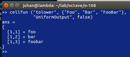
Function File: arrayfun (..., "UniformOutput", val)
Function File: arrayfun (..., "ErrorHandler", errfunc)

Execute a function on each element of an array.
This is useful for functions that do not accept array arguments. If the function does accept array arguments it is better to call the function directly.
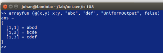
The first input argument func can be a string, a function handle, an inline function, or an anonymous function. The input argument A can be a logic array, a numeric array, a string array, a structure array, or a cell array. By a call of the function arrayfun all elements of A are passed on to the named function func individually.
The named function can also take more than two input arguments, with the input arguments given as third input argument b, fourth input argument c, ... If given more than one array input argument then all input arguments must have the same sizes, for example:

o596

If the parameter val after a further string input argument "UniformOutput" is set true (the default), then the named function func must return a single element which then will be concatenated into the return value and is of type matrix. Otherwise, if that parameter is set to false, then the outputs are concatenated in a cell array. For example:

o597

If more than one output arguments are given then the named function must return the number of return values that also are expected, for example:

o598

If the parameter errfunc after a further string input argument "ErrorHandler" is another string, a function handle, an inline function, or an anonymous function, then errfunc defines a function to call in the case that func generates an error. The definition of the function must be of the form function [...] = errfunc (s, ...) where there is an additional input argument to errfunc relative to func, given by s. This is a structure with the elements "identifier", "message", and "index" giving, respectively, the error identifier, the error message, and the index of the array elements that caused the error. The size of the output argument of errfunc must have the same size as the output argument of func, otherwise a real error is thrown. For example:

o599

Function File: y = spfun (f, S)
Compute f(S) for the nonzero values of S.
This results in a sparse matrix with the same structure as S. The function f can be passed as a string, a function handle, or an inline function.

o600

per contro

o601

Built-in Function: cellfun (name, C)
Built-in Function: cellfun ("size", C, k)
Built-in Function: cellfun ("isclass", C, class)
Built-in Function: cellfun (func, C)
Built-in Function: cellfun (func, C, D)
Built-in Function: [a, ...] = cellfun (...)
Built-in Function: cellfun (..., "ErrorHandler", errfunc)
Built-in Function: cellfun (..., "UniformOutput", val)

Evaluate the function named name on the elements of the cell array C.
Elements in C are passed on to the named function individually. The function name can be one of the functions

  • isempty Return 1 for empty elements.
  • islogical Return 1 for logical elements.
  • isnumeric Return 1 for numeric elements.
  • isreal Return 1 for real elements.
  • length Return a vector of the lengths of cell elements.
  • ndims Return the number of dimensions of each element.
  • numel, prodofsize Return the number of elements contained within each cell element. The number is the product of the dimensions of the object at each cell element.
  • size Return the size along the k-th dimension.
  • isclass Return 1 for elements of class.

Additionally, cellfun accepts an arbitrary function func in the form of an inline function, function handle, or the name of a function (in a character string). The function can take one or more arguments, with the inputs arguments given by C, D, etc. Equally the function can return one or more output arguments. For example:

o602

The number of output arguments of cellfun matches the number of output arguments of the function. The outputs of the function will be collected into the output arguments of cellfun like this:

o603

Note that per default the output argument(s) are arrays of the same size as the input arguments. Input arguments that are singleton (1x1) cells will be automatically expanded to the size of the other arguments.
If the parameter "UniformOutput" is set to true (the default), then the function must return scalars which will be concatenated into the return array(s). If "UniformOutput" is false, the outputs are concatenated into a cell array (or cell arrays). For example:

o604

Given the parameter "ErrorHandler", then errfunc defines a function to call in case func generates an error. The form of the function is function [...] = errfunc (s, ...) where there is an additional input argument to errfunc relative to func, given by s. This is a structure with the elements "identifier", "message" and "index", giving respectively the error identifier, the error message, and the index into the input arguments of the element that caused the error. For example:

o605

Use cellfun intelligently. The cellfun function is a useful tool for avoiding loops. It is often used with anonymous function handles; however, calling an anonymous function involves an overhead quite comparable to the overhead of an m-file function. Passing a handle to a built-in function is faster, because the interpreter is not involved in the internal loop. For example:

a = {...}
v = cellfun (@(x) det (x), a); # compute determinants
v = cellfun (@det, a); # faster

Function File: structfun (func, S)
Function File: [A, ...] = structfun (...)
Function File: structfun (..., "ErrorHandler", errfunc)
Function File: structfun (..., "UniformOutput", val)

Evaluate the function named name on the fields of the structure S. The fields of S are passed to the function func individually.
structfun accepts an arbitrary function func in the form of an inline function, function handle, or the name of a function (in a character string). In the case of a character string argument, the function must accept a single argument named x, and it must return a string value. If the function returns more than one argument, they are returned as separate output variables.
If the parameter "UniformOutput" is set to true (the default), then the function must return a single element which will be concatenated into the return value. If "UniformOutput" is false, the outputs are placed into a structure with the same fieldnames as the input structure.

o606

Given the parameter "ErrorHandler", errfunc defines a function to call in case func generates an error. The form of the function is function [...] = errfunc (se, ...) where there is an additional input argument to errfunc relative to func, given by se. This is a structure with the elements "identifier", "message" and "index", giving respectively the error identifier, the error message, and the index into the input arguments of the element that caused the error. For an example on how to use an error handler, see cellfun.

Consistent with earlier advice, seek to use Octave built-in functions whenever possible for the best performance. This advice applies especially to the four functions above. For example, when adding two arrays together element-by-element one could use a handle to the built-in addition function @plus or define an anonymous function @(x,y) x + y. But, the anonymous function is 60% slower than the first method. See Operator Overloading, for a list of basic functions which might be used in place of anonymous ones.

:mrgreen: